Home
Syllabus
Digital Audio, Part 1

Digital Audio, Part 1

Introduction to Digital Audio, Part 1

A Brief History

Earlier this semester, we studied some basic acoustics concepts — for example, that sound begins with the vibration of an object, which in turn creates patterns of compression and rarefaction of air molecules. It is just these changes in air pressure that are “captured” in both analog and digital recording methods.

In the 1870’s, Thomas Edison invented the phonograph, the first practical device capable of recording sound and playing it back. Over the next century, there were many innovations that improved sound recordings purchased by the typical consumer, but until compact discs became common in the 1980’s, most sound recordings were analog.

Analog to Digital Recording Chain

Digital recording always begins with a live acoustic pressure wave, as captured by a microphone; an analog electrical signal, such as a synthesizer audio output; or with an analog representation of sound already recorded on tape or phonograph (vinyl).

Sound made by bell transduced by microphone, then fed into ADC and finally to computer

In the illustration above, the bell is the live sound source. The microphone reacts to the acoustic energy created by the bell’s vibration (those changes in air pressure mentioned above), and converts the acoustic energy to electrical energy — a continuously changing voltage. For this reason, we say that the microphone is a transducer: it changes energy from one form to another.

The changes in electrical voltage mimic the shape or pattern of the acoustic waveform created by the bell, and so it is an analog of the bell’s waveform. Both the acoustic pressure changes and the analog electrical signal are continuously varying.

Next, the microphone’s signal is sent to an ADC, or Analog to Digital Converter. As you might guess by its name, the ADC converts the analog electrical signal to a digital signal.

The digital signal encodes the analog signal in binary numbers — zeroes and ones — that can be used and stored by your computer. However, we can’t listen to numbers. So those numbers must be converted back to an analog signal for your headphones. That task is accomplished by a DAC, or Digital to Analog Converter. The headphones (or speakers) transduce a continuously varying analog electrical signal into air pressure changes.

Analog Versus Digital

Here is a quick description of the difference between an analog sound signal and a digital sound signal:

Analog: a continuous signal that mimics the shape of an acoustic pressure wave
Digital: a stream of discrete numbers that represent instantaneous amplitudes of the analog signal, measured at equally spaced points in time

To visualize this important difference, it might help to think of the analog signal as similar to a ramp, while the digital signal, by contrast, is more like stair steps.

Continuous analog linear ascent versus stair-step digital ascent

Analog to Digital Conversion

Let’s discuss, in greater depth, how analog signals become digital signals. This illustration shows an analog electrical signal, such as a microphone emits, with its amplitude curve over time graphed as a red line.

Two cycles of a sine wave on a grid of equally spaced vertical lines

The gray vertical lines superimposed on the red waveform represent the equally spaced points in time when the amplitude of the waveform will be measured.

Two cycles of a sine wave with amplitude measurements, shown as blue stars, taken at equally spaced points in time

The amplitude measurements, or sample points, shown in the illustration above as blue stars, are like a series of snapshots that, taken together, describe the amplitude curve of the original acoustic waveform.

Analog to Digital Overview

There are two main characteristics of analog-to-digital conversion: sampling rate, which determines the range of frequencies that can be encoded; and sampling resolution — the accuracy of amplitude measurements — which determines the level of noise in the digital signal.

Sampling Rate: how often analog signal is measured — expressed in samples per second (Hz)
Example: 44,100 Hz
Sampling Resolution: accuracy of numbers used for amplitude measurement: the more bits, the higher the resolution — also known as “sample word length,” and “bit depth”
Example: 16 bit

In the illustration above, the sampling rate is shown by the gray vertical lines: the higher the sampling rate, the closer together those lines will be.

Sampling resolution is the main subject of Digital Audio, Part 2.

The Nyquist Theorem

The sampling rate determines the highest frequency you can represent with a digital signal. The Nyquist Theorem (named after the Swedish-born researcher, Harry Nyquist) states that...

the sampling rate must be at least twice as high as the highest frequency you want to represent.

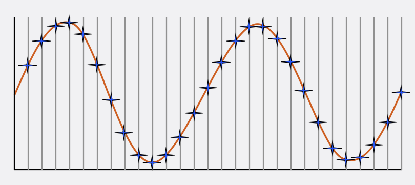
One way to think about this is to imagine a high-frequency sine wave for which we sample exactly two points per cycle: the crest (top) of the waveform, and the trough (bottom) of the waveform.

Two cycles of a sine wave, each with one sample at the top and one at the bottom of the cycle

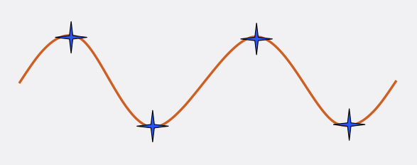
The illustration shows two cycles of a sine wave, with each cycle represented by two sample points (the blue stars).

The sample points shown are sufficient to allow us to reconstruct the original analog audio signal. Since there are two sample points for each cycle, that means that the sampling rate (or frequency) is twice the frequency of the sine wave. (So if the sine wave is 10,000 Hz, the sampling rate is 20,000 Hz.) That fits with the requirement of the Nyquist Theorem that the sampling rate be at least twice as high as the highest frequency in the signal.

The frequency shown above is critically sampled, meaning that if you had any fewer sample points per cycle, you would not be able to represent the analog signal accurately. This frequency, which is exactly half of the sampling rate, is called the Nyquist frequency.

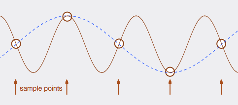
(You might be skeptical about the claim, made above, that two samples points per cycle allows you to reconstruct the sine wave. Wouldn’t a reconstruction create straight lines between the points? In fact, the process of converting a digital signal back to analog form includes an analog “smoothing” filter that causes the output to closely approximate the original curved shape.)

Aliasing

What would happen if the sampling rate were not high enough? You would hear an artifact called aliasing, or foldover: a high frequency signal sampled at too low a rate will “masquerade” as a lower frequency signal.

A sine wave with fewer than two samples per cycle aliases as a lower-frequency sine wave

The illustration shows an analog signal in red, sampled at the places that are circled. This sine wave has a frequency that is higher than the Nyquist frequency. Because there are fewer than two sample points per cycle of the red sine wave, aliasing occurs. The dashed blue curve shows the sine wave that is represented by the given sample points. This sine wave alias has a frequency that is 1/3 as high as the original red sine wave. If the sampling rate were 20,000 Hz, then the Nyquist frequency would be 10,000 Hz. In this case, the red sine is 15,000 Hz, too high to be represented correctly. Instead, it “folds over” to 5000 Hz. (You will not be responsible for calculating such things on a quiz.)

An ADC has an analog low-pass anti-aliasing filter to solve this problem: it filters out frequencies that are above the Nyquist frequency before analog-to-digital conversion happens. However, software that synthesizes audio can cause aliasing by generating frequencies that are higher than the Nyquist frequency. These high frequencies alias as lower frequencies after digital-to-analog conversion. There is no way to filter out these spurious alias frequencies after they’ve been generated. Some software has anti-aliasing oscillators to keep this from happening in many cases.

Below, you can play an upward sine wave glissando from 20 Hz to 44,100 Hz, converted from digital to analog at a sampling rate of 44,100 Hz. Wait a bit after you hear the pitch get so high that it disappears. Once the glissando crosses the Nyquist frequency (22,050 Hz), the pitch will “fold over,” reappear, and drop to the bottom again — even though the frequency of the digital signal is still rising to 44,100 Hz.

Continuous glissando from 0 to 44,100 Hz.

Common Sampling Rates

In class, we will listen to examples of a recording captured at several several different sampling rates.

The most common sampling rates are:

44,100 Hz (CD)
48,000 Hz (DV, DVD-Video)
96,000 Hz (current external audio interfaces)

Why would a 96,000 Hz sampling rate be useful, if humans can hear nothing beyond 20 kHz? Actually, some people believe that humans can sense these higher frequencies. But the better reason is that making the sampling rate so high allows converter designers to create anti-aliasing filters that have a flatter frequency response across the spectrum from 0 to 20,000 Hz.